How To Add Filter In Excel Pivot Table

Add filter option for all your columns in a pivot table. The next line of code do just that.

Filtering Excel Pivot Tables With A Timeline Pivot Table Create A Timeline Excel

The State field is added as a Pivot Table filter.

How to add filter in excel pivot table. First create a table using a Pivot Table. On the worksheet Excel adds the selected field to the top of the pivot table with the item All. Select larger smaller than.

Sort previous post Excel could be a database with VLOOKUP next post Change the color of the weekends. In an empty cell to the right of the Pivot table create a cell to hold the filter and then type the data into the cell that you wish to filter the Pivot table on. Here we have an empty pivot table using the same source data weve looked at in previous videos.

Convert pivot table to worksheet. Please click the arrow beside All check Select Multiple Items option in the drop-down list next check dates you will filter out and finally click the OK button. Click on the Label filter drop down and then click on the search box to place the cursor in it.

Add a column from the Date table to the Column Labels or Row Labels area of the Power Pivot field list. In that drop-down list we have traditional filter options. Select of specific values.

To do this we have to select any cell inside of our pivot table here and go over to the pivot table field list and going to remove Industry from the rows removing Count of Age Category from the values area and we are going to take the Function that is in our filters area to rows area and so now we can see that we have a list of our filter criteria if we look over here in our filter drop-down menu we have the list of item that is there in slicers and function filter. Enter the search term which is dollar in this case. Click on the drop-down arrow or press the ALT Down navigation key to go into the filter list.

Point to Date Filters and then select a filter from the list. Click the down arrow next to Column Labels or Row Labels in the PivotTable. Just click the down arrow beside Row Labels in the pivot table then select the field you want to filter based on from the Select field list.

In the PivotTable Field list click on the field that you want to use as a Report Filter. To clear the filter create the following macro. Navigate to a PivotTable or PivotChart in the same workbook.

Colbrawl Try by right-clicking on any of the row labels of your pivot table. Two table headers Name and City are added to the Rows Field. The filter will then be removed.

Lets take a look. Years has been added as a Column field and Date Quarters has been added as a Row field. Here you can set the filter to your liking.

It should open a window where you can select Filter and then Value Filters. Drag the field into the Filters box as shown in the screen shot below. Pivot table group by quarter Exceljet.

Browse to and open the workbook file containing the pivot table and source data for which you need filter data. Determine the attribute by which you want to. Youll notice that the list gets filtered in the below the search.

Finally the Sales field has been added as a Value field and set to Sum values. We can see the first field which is either a Row or Column will have one filter. Select the worksheet containing the pivot tab and make it active by clicking the appropriate tab.

Choose between and provide the lower and upper bounds. Here are the steps. After grouping the Years field appears in the field list and the Date field displays quarters in the form Qtr1 Qtr2 etc.

Lets add product as a row label and add. Run the macro to apply the filter. Now City is after Name but its important to have City as the first position.

In addition to filtering a pivot table using row or column labels you can also filter on the values that appear inside the table. Go to the pivot table you will see the Date field is added as report filter above the pivot table. The last line before the end is xlHiddenField.

Create the following VBA macro.

What Is An Excel Pivot Table In 2021 Pivot Table Excel Tutorials Excel Pivot Table

How To Create A Calculated Item In An Excel Pivot Table Excel Pivot Table Computer Jobs

Excel Pivot Tables Tutorial What Is A Pivot Table And How To Make One Pivot Table Excel Tutorial

Pin On Pivot Table Tips

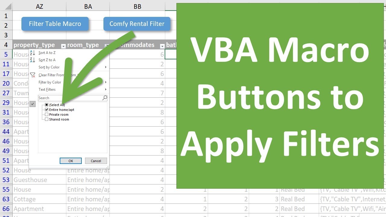
107 How To Create Macro Buttons For Filters In Excel Youtube Online Student Excel Data Science

Learn Excel Pivot Table Slicers With Filter Data Slicer Tips Tricks Pivot Table Excel Learning

How To Use Excel Pivot Tables To Organize Data Pivot Table Excel Organization

Excel Pivot Tables Tutorial What Is A Pivot Table And How To Make One Pivot Table Excel Pivot Table Tutorials Excel Pivot Table

Pin On Excel

50 Things You Can Do With Excel Pivot Table Myexcelonline Excel Tutorials Pivot Table Excel

Excel Pivot Tables Pivot Table Pivot Table Excel Excel Tutorials

Pivot Table Super Tips In Excel Search Box In Slicer Cross Filter In Two Pivot Tables Youtube Excel Tutorials Pivot Table Excel

The Ultimate Guide On Excel Slicer Myexcelonline Excel For Beginners Microsoft Excel Tutorial Excel Tutorials

In This Video We Look How Slicers Filter Data In A Pivot Table And How To Easily Add A Slicer To A Pivot Table Pivot Table Ads Excel

Make A Pivot Table Timeline In Excel Tutorial Excel Tutorials Pivot Table Microsoft Excel Tutorial

Add A Search Box To The Slicer To Filter It Quickly Pivot Table Keyboard Shortcuts Workbook

Pivot Table Errors Pivot Table Excel Formula Pivot Table Excel

Follow These Easy Steps To Create A Pivot Table In Microsoft Excel 2016 Excel Pivot Table Microsoft Excel Tutorial

50 Things You Can Do With Excel Pivot Table Myexcelonline Excel Tutorials Excel Excel Shortcuts