How To Add Multiple Values In Excel Chart
Apply data labels to series 2 outside end. Then in Format Data Series dialog check.
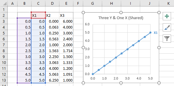
Multiple Series In One Excel Chart Peltier Tech
How To Add A Column In Pivot Table 14 S With Pictures.

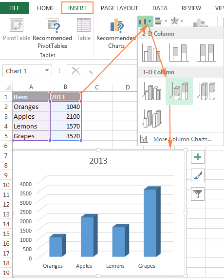
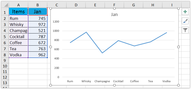
How to add multiple values in excel chart. As shown below cells A2A5 contain the data Items. You can see the below chart. Group two-level axis labels with adjusting layout of source data in Excel.
Assuming youre using Excel 2007 data labels are added through the Data Labels selection. Pivot Table Basic Sum Exceljet. Add Multiple Columns To.
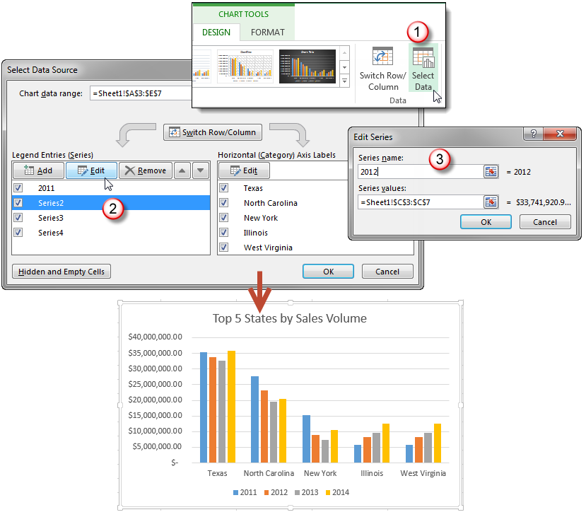
Select the chart area and click on the button that pop-up at its right once you click the same. Or click the Chart Filters button on the right of the graph and then click the Select Data link at the bottom. Add Multiple Columns To A Pivot Table Custom.
Adjust series 2 data references Value from B2D2. Apply data labels to series 1 inside end. Make two y axis in chart.
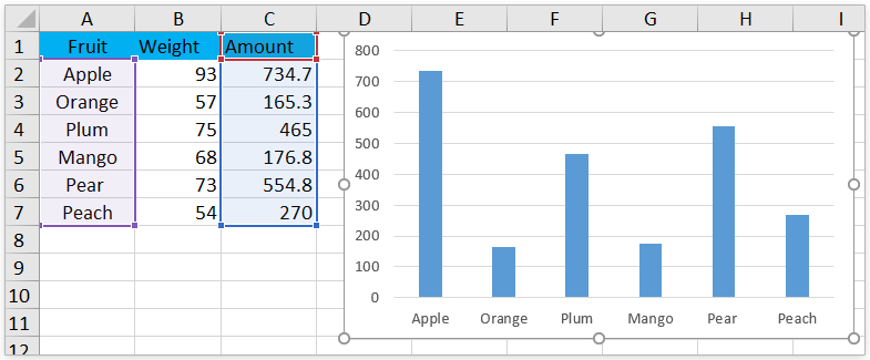
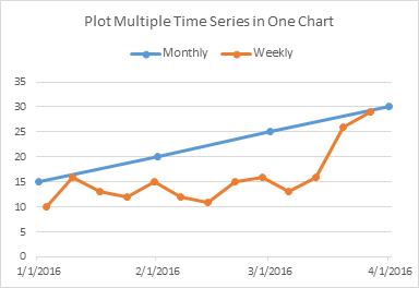
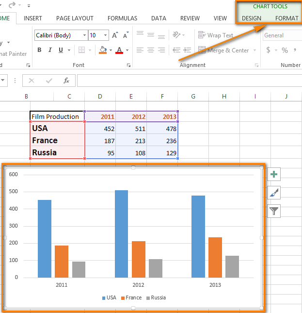
This displays the Chart Tools adding the Design Layout and Format tabs. Select the fruit column except the column heading. Select and copy the weekly data set select the chart and use Paste Special to.
Pivot Table With Text In Values Area Excel Mrexcel Publishing. 4 Click on the graph to make sure it is selected then select Layout. Select Series Data.
Right click the chart and choose Select Data or click on Select Data in the ribbon to bring up the Select Data Source dialog. Right click a column in the chart and select Format Data Series in the context menu. Insert the data in the cells.
Select 2 series diff base line and move to secondary axis. Add a data series to a chart on a separate chart sheet. Select A1D4 and insert a bar chart.
Comparison Chart in Excel Adding Multiple Series. You cant edit the Chart Data Range to include multiple blocks of data. From the pop-down menu select the first.
In a chart click the data series that you want to plot on a secondary vertical axis or do the following to select the data series from a list of chart elements. Category labels from B4D4. Cells B2B5 contain the data Values.
Select the data range and insert a chart first by clicking Insert and selecting a chart you need in the Chart group. To create a combo chart select the data you want displayed then click the dialog launcher in the corner of the Charts group on the Insert tab to open the Insert Chart dialog box. On the worksheet that contains your chart data in the cells directly next to or below your existing source data for the chart enter the new data.
Excel Pivot Tables Summarizing Values. 1 Select cells A2B5. In our case please select the Range A2A17 and then.
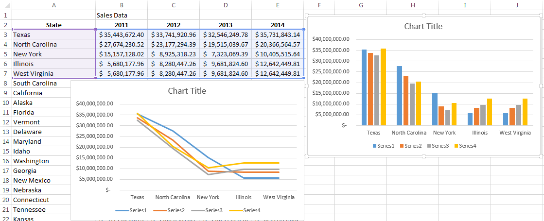
Click on the chart youve just created to activate the Chart Tools tabs on the Excel ribbon go to the Design tab and click the Select Data button. After selecting the data as mentioned above and selecting a stacked column chart. Select combo from the All Charts tab.
Now click on Insert Tab from the top of the Excel window and then select Insert Line or Area Chart. Select 2 series and delete it. Choose the stacked column stack option to create stacked column charts.
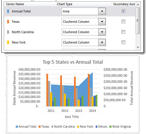
Select the chart type you want for each data series from the dropdown options. Click the worksheet that contains your chart. Excel has detected the dates and applied a Date Scale with a spacing of 1 month and base units of 1 month below left.
In Column chart options you will see several options. After insertion select the rows and columns by dragging the cursor. Right-click the chart and then choose Select.
Start by selecting the monthly data set and inserting a line chart. Move the fruit column before Date column with cutting the fruit column and then pasting before the date column. However adding two series under the same graph makes it automatically look like a comparison since each series values have a separate barcolumn associated with it.
In this video I show you how to copy the same chart multiple times and then change the cell references it is linked to in order to make lots of similar chart. Click on Insert and then click on column chart options as shown below. However you can add data by clicking the Add button above the list of series which includes just the first series.
2 Select Insert 3 Select the desired Column type graph.
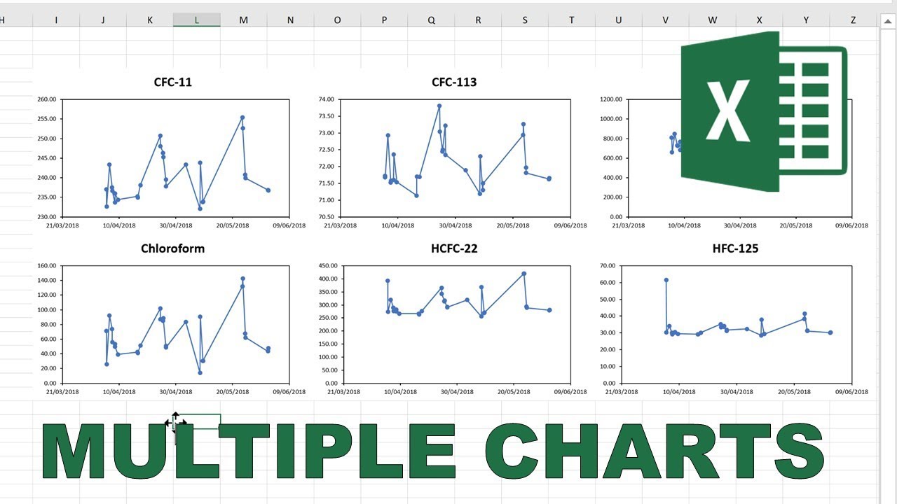
How To Quickly Make Multiple Charts In Excel Youtube
Plot Multiple Lines In Excel Youtube
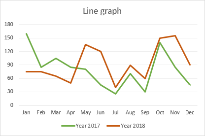
How To Make A Line Graph In Excel

How To Create A Chart By Count Of Values In Excel
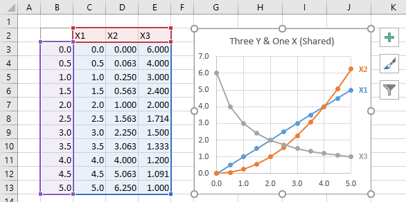
Multiple Series In One Excel Chart Peltier Tech
Working With Multiple Data Series In Excel Pryor Learning Solutions
How To Create A Chart In Excel From Multiple Sheets
How To Add Comment To A Data Point In An Excel Chart
Multiple Time Series In An Excel Chart Peltier Tech
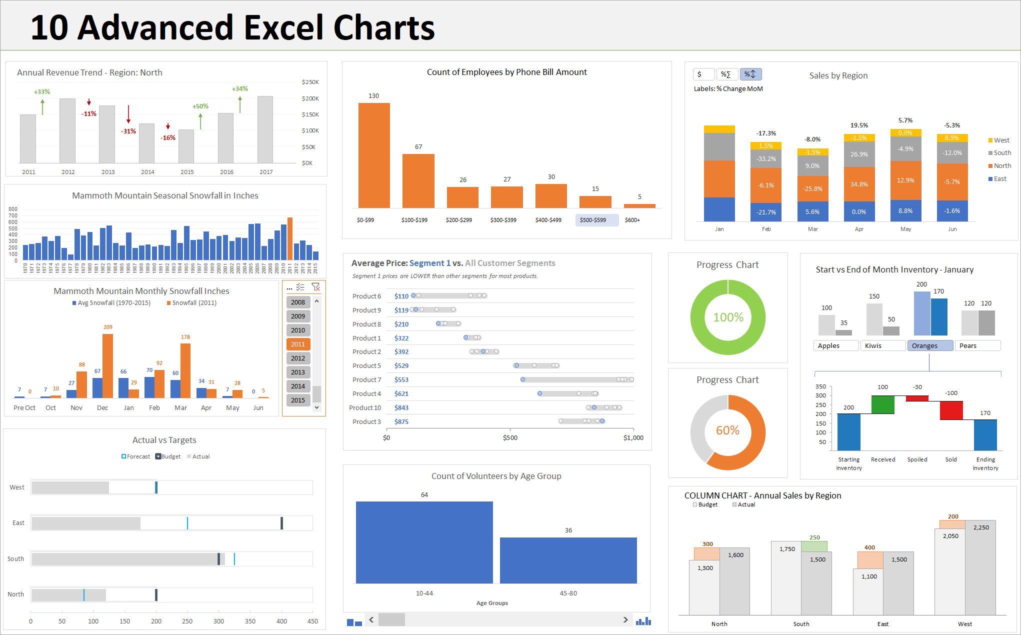
10 Advanced Excel Charts Excel Campus
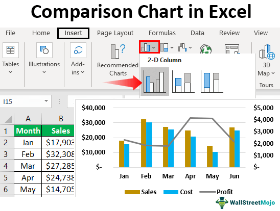
Comparison Chart In Excel How To Create A Comparison Chart In Excel
Multiple Series In One Excel Chart Peltier Tech
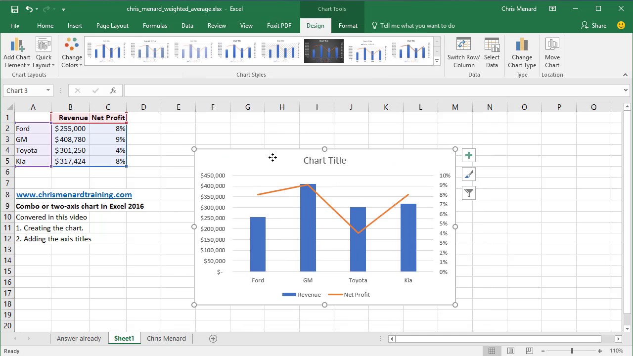
Create A Combo Chart Or Two Axis Chart In Excel 2016 By Chris Menard Youtube
How To Add A Single Data Point In An Excel Line Chart

Multiple Series In One Excel Chart Peltier Tech
How To Add Titles To Excel Charts In A Minute
Working With Multiple Data Series In Excel Pryor Learning Solutions
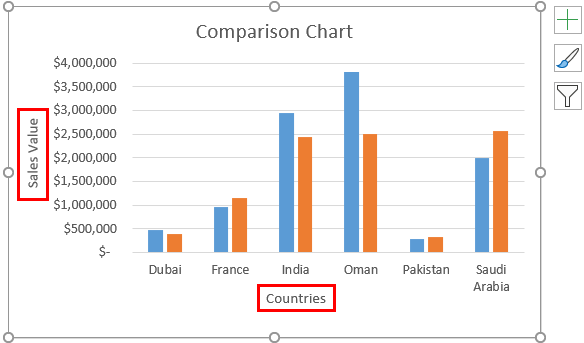
Comparison Chart In Excel Adding Multiple Series Under Same Graph
Working With Multiple Data Series In Excel Pryor Learning Solutions