How To Total In Excel With Filter
Show Or Hide Total Values On A Chart How To Visualizations Doentation Learning. If you used the SUM function in the grand total cell the result wont change if a filter is.

Set Up The Following Ranges Similar To What You Would Use For An Advanced Filter A Database Range A Criteria Range In This Example The Sum Ms Office Excel
If some extra rows arrows are selected you can press CTRL SHIFT Up Arrow to adjust the same.
How to total in excel with filter. Next we need to count the number of visible rows. To count total rows we can use the function ROWS and simply input ROWS Properties. After that select the cell immediately below the column you want to total and click the AutoSum button on the ribbon.
Create a SUBTOTAL formula. How to Excel 365 Filter with indirect array of addresses not continuous. Just organize your data in table Ctrl T or filter the data the way you want by clicking the Filter button.
Save this code and enter the formula SumVisible C2C12 into a blank. Click Insert Module and paste the following code in the Module window. By selecting the entire data set pressing CTRL SHIFT Right Arrow and then CTRL SHIFT Down Arrow.
Reading a SUBTOTAL formula. Click anywhere inside the table. If you apply formulas to a total row then toggle the total row off and on Excel will remember your formulas.
The formula below has the same result as above with red hardcoded into the criteria. You can see there is no change in the totals. The solution is much easier than you might think.
This is a structured reference that refers only to the data rows in the Properties table which is ideal for this use. Values can be hardcoded as well. While filtering you must keep in mind that checkbox nex to the required name is only checked.
This is because we have used the SUM Function. Now if you wanted to find the sales total you can use the following formula. If you remember from last weeks blog post on Sorting and Filtering data we have gone ahead and added the filter.
Then press Enter key to get the total value and now if you filter this data the total row will be excluded and. In this case were using the FILTER function with the addition operator to return all values in our array range A5D20 that have Apples OR are in the East region and then sort Units in descending order. Apply a filter to the list.
The Total Row is inserted at the bottom of your table. FILTERINDIRECTM2N2O2P2Q2R2 INDIRECTM2N2O2P2Q2R2 Intermediate Formula Evaluation shows. We want to populate column D with a cumulative total that will work when the sheet is filtered by the Department in column B.
If you filter after applying the SUM function you will still see the total including the data hidden by the filter. Trick To Show Excel Pivot Table Grand Total At Top. How To Add Average Grand Total Line In A Pivot Chart Excel.
Total a Filtered List in Excel SUM Function Problem. To do this well use the SUBTOTAL function. Add Totals To Stacked Bar Chart Peltier Tech.
Go to Table Tools Design and select the check box for Total Row. FILTER B5D14 D5D14 redNo results To return nothing when no matching data is found supply an empty string for if_empty. In this example the Region column is filtered for West.
SUM C2C50 Lets filter the table for a particular customer say Abhishek Cables. Sum range This is the standard way to find a total. SORT FILTER A5D20 C5C20H1 A5A20H24-1.
Add Totals To Stacked Column Chart Peltier Tech. The formula for cell D2 is AGGREGATE 95C1C2 This formula can be copied down. 1 2 3 4 5 6 7 8 9 10 11 Function SumVisible.
If you wouldnt like to create a table the SUBTOTAL also can do you a favor please do as follows. FILTER B5D14 D5D14 H2. You can have Excels AutoSum feature to insert the Subtotal formula for you automatically.
SUBTOTAL 9B2B13 into the bottom row see screenshot. Firstly Apply a filter to your data set. Hold down the ALT F11 keys and it opens the Microsoft Visual Basic for Applications window.
The first thing you will need to do is apply Filter to your data and then be sure to have the data filtered BEFORE trying to SUM the range. Simply click AutoSum-- Excel will automatically enter a SUBTOTAL function instead of a SUM function. Ms Excel 2016 How To Remove Row Grand Totals In A Pivot Table.

How To Save Filter Criteria In Microsoft Excel Excel Filter Excel Tutorials Excel Microsoft Excel

Follow These Easy Steps To Create A Pivot Table In Microsoft Excel 2016 Excel Pivot Table Microsoft Excel Tutorial

23 Things You Should Know About Excel Pivot Tables Via Exceljet Pivot Table Excel I Need A Job

Multi Level Pivot Table In Excel Pivot Table Excel Microsoft Excel

Add A Search Box To The Slicer To Filter It Quickly Pivot Table Keyboard Shortcuts Workbook

Set Up The Following Ranges Similar To What You Would Use For An Advanced Filter A Database Range A Criteria Range In This Example Excel Workbook New Names

5 Best Ways To Manage Inventory In Excel Spreadsheet Template Spreadsheet Excel

8 Pivot Table Problems Solved Easily Pivot Table Problem Solving Excel Formula

Excel Formula Sum Time With Sumifs Excel Formula Getting Things Done Sum

How To Filter Data In A Pivot Table In Excel Pivot Table Excel Pivot Table Excel

Count Number Of Months For A Period Longer Than A Year Excel Years Months

Excel Table How To Format Excel Tables With Total Sort And Filter Here Are A Few Basics On Excel Formatting Read On To Data Logo Google Interactive Sorting

Multi Level Pivot Table In Excel Pivot Table Excel Tutorials Learning Tools

Filter Columns With Slicer Macro Quarterly Report Example Excel Column Filters

Filter Records Excel Formula Sorting By Color Excel
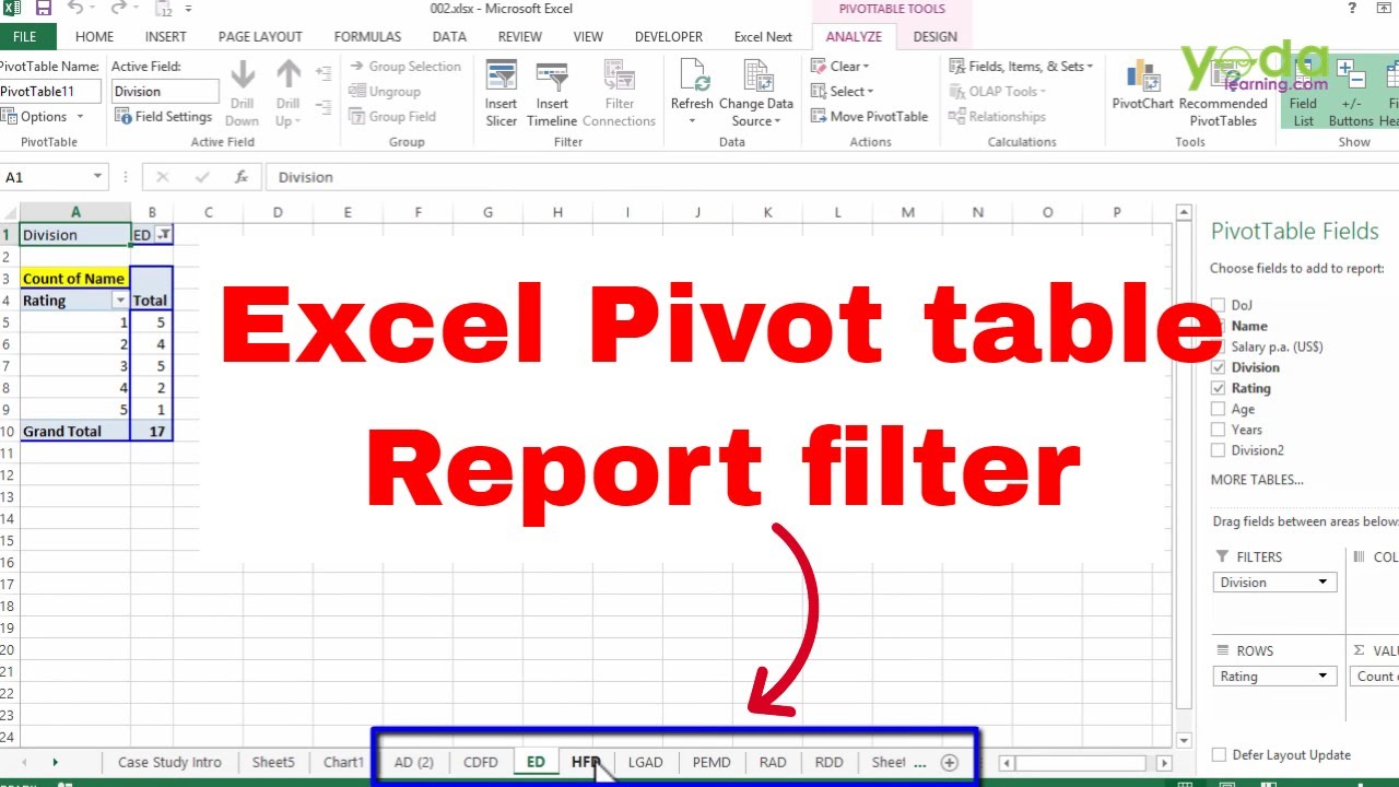
Excel Pivot Table Report Filter Advanced Excel Youtube Pivot Table Excel Tutorials Pivot Table Excel

Learn Excel Pivot Table Slicers With Filter Data Slicer Tips Tricks Pivot Table Excel Table Topics

Multi Level Pivot Table In Excel Excel Pivot Table Microsoft Excel

Excel Vba Macros Sql Examples Tutorials Free Downloads How To Sort Pivot Table Row Labels Column Field L Excel Pivot Table Sorting