How To Show Total Value In Excel Chart

31 Aug, 2021

Select the totals column and right click. Extra settings to change the color and X Y.

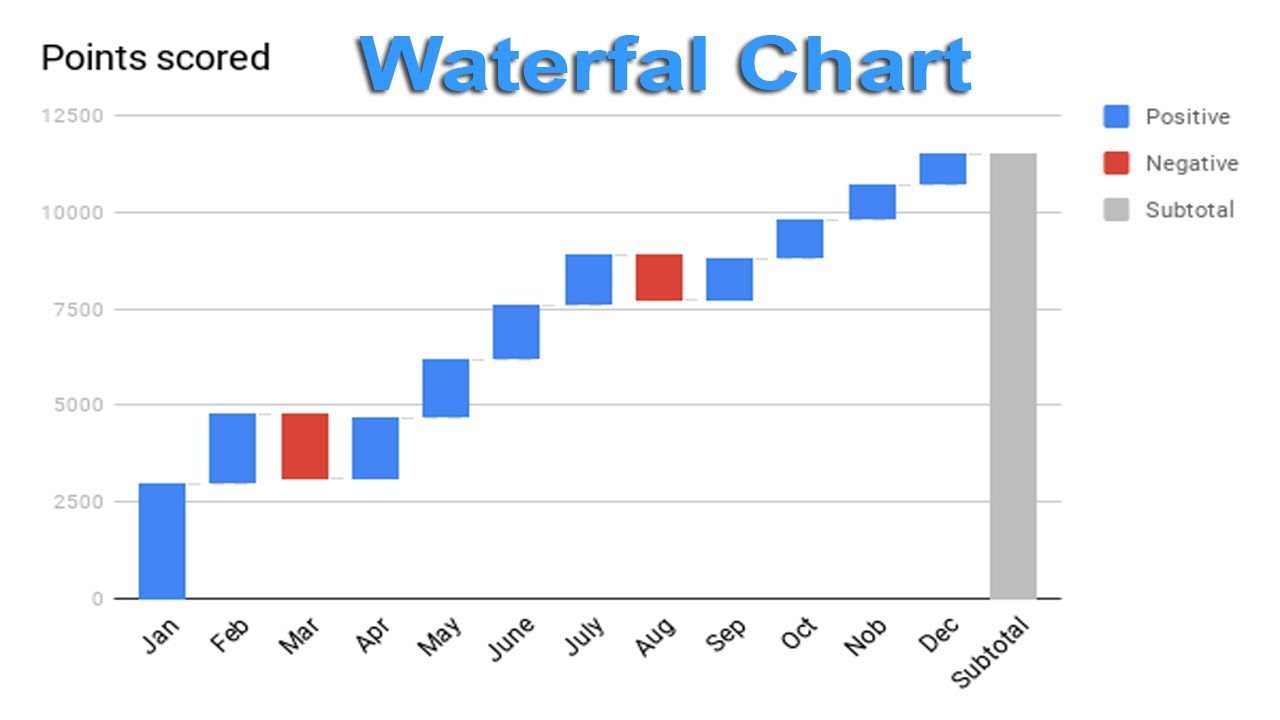
How To Create Waterfall Chart Graph In Google Docs Chart Charts And Graphs Graphing

Excel Pivot Table Chart Add Grand Total Bar.

How to show total value in excel chart. Right click on the series or on any series and select Change Series Data Type then find the series and in the chart type dropdown select the type you need. Select the data range that you want to create a chart but exclude the percentage column and then click Insert Insert Column or Bar Chart 2-D. By clicking on the title you can change the tile.

Then convert the added series to a line chart series type below right. Select data for the chart. Then insert a text box on top of the chart Insert Picture Autoshapes.

Click on the Insert tab. Change the Spacing column values to a number eg 1000 big enough to make a new category visible on the stacked bar chart. In the Select Data Label Range pop up box highlight the values from the Grand Total column.

4 Click on the graph to make sure it is selected then select Layout. Select the textbox and in the formula bar type Sheet1A5 The textbox will be linked to that cell. Another way to add a total row in Excel is to right click any cell within the table and then click Table Totals Row.

Create a chart with both percentage and value in Excel. 1 Select cells A2B5. Right-click Option You simply need to isolate the value or column you want to set as a total by clicking on it.

Show Or Hide Subtotals And Totals In A Pivottable Office Support. Select a blank cell adjacent to the Target column in this case select Cell C2 and type this formula SUM B2B2 and then drag the fill handle down to the cells you want to apply this formula. After inserting the chart then you should insert two helper columns in the first.

In order to add a chart in Excel spreadsheet follow the steps below. Then right-click and navigate down to the section for setting a total as shown in the above picture. If your data includes values that are considered Subtotals or Totals such as Net Income you can set those values so they start on the horizontal axis at zero and dont float.

Lab 6 Part 1 Pivot Table Tables Are One Of Excel S Most Powerful Features A Allows You To Extract The Significance From Large Detailed Set Lab6pivot Xlsx Announcement Page Consists 214. Add A Running Total Column Excel Pivot Table. Change Chart type dialog will open.

SUMA1A4 or something like that to cell A5-. Here you can see all series names Delhi Mumbai Total and Base Line. Httpbitly2pnDt5FLearn how to add total values to stacked charts in ExcelStacked charts are great for when you want to compa.

Click on Change Series Chart Type. The chart will be inserted for the selected data as below. You can add a label to it too to by entering Total.

3 Select the desired Column type graph. We will look at a full example below. Select the data and go to the chart option from the Insert menu.

How to total data in your table. 5 Select Data Labels Outside End was selected below If you dont want the Values as the Labels you can click on the desired label click. Click anywhere in the table to display the Table Tools with the Design tab.

Click on the Recommended Charts. Right click to Format Data Labels and change the Label Options to Value from Cells. Download the workbook here.

Open MS Excel and navigate to the spreadsheet which contains the data table you want to use for creating a chart. On the Design tab in the Table Style Options group select the Total Row box. Click on the bar chart select a 3-D Stacked Bar chart from the given styles.

Start subtotals or totals from the horizontal axis. Excel seems to have a way to do this by right clicking on the table selecting Pivot Chart Options - Totals Filters - Show grand totals for columns but nothing happens when I do this so not sure how its supposed to function. Create an accumulative sum chart in Excel 1.

The easiest way is to select the chart and drag the corners of the highlighted region to include the Totals. Double-click a data point to open the Format Data Point task pane and check the Set as. Cells B2B5 contain the data Values.

If the type of calculation of the value field Fruit is not Count please click Fruit in the Values section Value Field Settings next in the Value Filed Setting dialog box click to highlight Count in the Summarize value filed by section and click the OK button.

Excel Pivot Tables Custom Calculations Pivot Table Free Workbook Excel Spreadsheets

Burndown Chart Generator Excel Chart Excel Templates Gantt Chart Templates

Sum Values Between Two Dates With Criteria In Excel Dating Payroll Template Sum

Show Chart Data In Hidden Cells Chart Excel Data

Pin On Excel

Pin On Excel Charts Collection

Errors In Excel Pivot Table Grand Totals But No Errors In Column Pivot Table Excel Tutorials Excel

Formatting Secondary Vertical Axis Chart Tool Column Create A Chart

Water Fall Chart Shows The Cumulative Effect Of A Quantity Over Time It Shows The Addition And Subtraction In A Basic Val Chart Excel Addition And Subtraction

Show Or Hide Subtotals And Totals In A Pivottable Excel Column Labels